
What is an average?
Study results are nearly always based on finding a pattern from lots of individual observations. In order to see any trend, the average of these observations is presented in the study report.
The average can be used to be able to generalise results for larger groups of people or larger sets of results.
You always need to remember when looking at average results that some results will have been higher and lower than the average. This is especially important when looking at studies related to healthcare.
Mean and median
The two most common ways used ways to calculated the average can give very different results.
Mean average
This is where all the results are added together, and then divided by the number of results to find the average.
So, CD4 increases after 6 months’ treatment in 10 people could be:
+20, +40, +15, -20 , -5, +120, +250, +30 ,+50, +100
Most people had increase but some peoples count was lower after 6 months.
The mean from these results would be 20 + 40 + 15 -20 etc divided by 10 people:
The mean average for this sample is 600 divided by 10 = 60.
Median average
This is where the results are all arranged in numerical order and the middle of the range is taken as the average.
So, CD4 increases after 6 months treatment in the same 10 people would be:
-20, -5, +15, +20, +30, +40 ,+50, +100, +120, +250
The median CD4 increase would be the middle point – half way between the 5th and 6th result:
The median for this sample is +35.
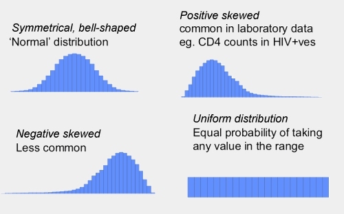
Data ‘shapes’

Even distribution is a term to describe data where most results are in the middle and a roughly similar number of results fall either side. It is also called a bell-shaped or ‘normal’ distribution . If results are evenly distributed then the mean average should be used
When the results are unevenly distributed this is called a skewed distribution. For example the majority of results may be higher or lower than the middle range and skewed to the right (negative skewed, less common) or the left (positive skewed, common in lab data). In these cases it is important to use the median average.
- In the example above, the CD4 count of one person that was much higher than the rest (+250) – this had a disproportionate effect on the mean average.
- The mean of 48 + 49 + 50 + 50 + 51 + 52 is 300/6 = 50
- But the mean of 0 + 25 + 50 + 50 + 75 + 100 is also 300/6 = 50
You can see that completely different patterns of results give you the same mean average.
Showing variations
Different ways to show variation are used depending on whether the results are evenly or unevenly distributed.
Even distribution
If distribution is even and you are using the mean average, then variation is usually calculated as being twice the standard deviation – and shown in brackets with a +/- sign in front of the result.
- 1 times standard deviation gives you the middle range of 50% of the results.
- 2 times standard deviations give you the middle range of 95% of the results.
- A standard deviation of 2 means 95% of the results are very close to the average.
- A standard deviation above 5 means the results are very far from the average.
Uneven distribution
If distribution is uneven – like the example of CD4 counts earlier – and you are using the median average, variation is easier to understand and shown in two main ways:
1. Showing the lowest and the highest results (the range of results):
- Sample: -20, -5, +15, +20, +30, +40, +50, +100, +120, +250
- Median: 35 (range -20, +250)
2. Using the middle half of the results (called the Inter Quartile Range or IQR):
- Sample: -20, -5, +15, +20, +30, +40, +50, +100, +120, +250
- Median: 35 (IQR 10, 110)
This is the range of the middle 50% of result with the highest 25% and lowest 25% not included.
The Inter-Quartile Range is sometimes given instead of the full range to reduce the impact of very high or very low results.
Last updated: 22 July 2009.